35 posts tagged with "Apache Iceberg"

Conventional wisdom says migrating a data engine to ARM is a performance gamble you take for the discount. We ran the experiment on our own Spark compute pools, and the result inverted the premise: under 100-way concurrency, the ARM64 pool ran every job roughly twice as fast as its x86 twin — at about 20% lower infrastructure cost.

We are publishing the numbers, but also the part benchmark posts usually cut: our first measurement said ARM was 8.5x slower, and that number was wrong in a way that had nothing to do with ARM. If you are planning an ARM migration for your data platform, the detour is probably worth more to you than the table.

In The Small Job Tax we made an argument: most data platforms make you pay cluster-sized overhead for container-sized work, and your smallest jobs are quietly your most expensive per byte.

An argument is cheap. So we measured it.

One hundred Spark jobs, submitted concurrently, each one scanning ~200 MB of Iceberg data — 19 GiB of real columnar IO and 410 million rows in total — finished in 67.5 seconds, on one small compute pool that costs about $2 an hour. One hundred submitted, one hundred succeeded, zero failures.

Then we kept pushing: 200 jobs, 300, 400, 500. The pool never became the problem.

There is a long-standing assumption in data engineering: if you want fast SQL, you do not use Spark. Spark is for pipelines. For interactive analytics you bring in a dedicated query engine, run it alongside, and accept the cost of operating two systems over one set of tables.

We wanted to know how true that still is. So we ran the full TPC-DS benchmark — all 103 queries — against a terabyte of Apache Iceberg data on a four-worker Cazpian cluster, and published everything: every query time, the cost, the hardware utilisation, and the parts that are not yet good enough.

Every native execution engine for Spark arrives with the same headline: 2x, 3x, sometimes 5x faster. The benchmarks are usually real. What they rarely tell you is whether they describe your data, your table format, and your version matrix.

So we measured it ourselves. Cazpian Native Query Acceleration, against 200 million rows of Apache Iceberg data, on the Spark version we ship. We recorded wall-clock time, CPU seconds, peak memory, and — the part most benchmarks skip — whether the answers came back the same.

The result: 1.51x faster on 45% less CPU across a mixed suite, with every result identical to standard Spark. On decimal aggregation — the shape most finance and revenue reporting takes — 3.18x in the suite, and 4.14x when we later measured it end to end through the Iceberg catalog.

We also nearly published the exact opposite conclusion. Our first full round measured zero acceleration on Iceberg — not "a little", literally zero accelerated operators across five configurations. That result was real, reproducible, and completely misleading, and the reason it was wrong is worth more to you than the speedup number.

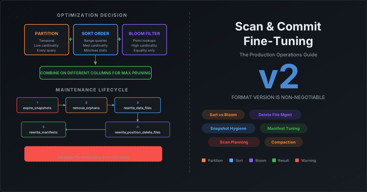
You have set up your Iceberg tables. You picked a partition spec. You enabled bloom filters. Maybe you even ran compaction once. But the questions keep coming: Should I sort the table AND add bloom filters, or is one enough? My queries are still opening thousands of files — what is Spark actually doing during scan planning? I have 50,000 snapshots — is that a problem? I switched to format version 2 but my reads got slower — why? What happens if I never compact my delete files?

These are the questions that every data engineering team hits after the first month in production. The individual features are documented, but the interactions between them — and the operational decisions that determine whether your tables stay fast or silently degrade — are not written down anywhere.

This post is the production operations guide. We cover the decision framework for partition vs sort vs bloom filter, explain exactly what happens during scan planning so you know where compute is wasted, walk through every maintenance procedure with recommended thresholds, explain why format version 2 is non-negotiable and what delete file neglect costs you, and give you the complete maintenance lifecycle in the right execution order.

You tuned your Spark cluster. You picked the right join strategies. You enabled AQE. But you are still flying blind. When a job takes twice as long as yesterday, you open the Spark UI, scroll through 200 stages, and guess. When an Iceberg scan suddenly plans for 12 seconds instead of 2, you have no history to compare against. You cannot trend what you do not collect.

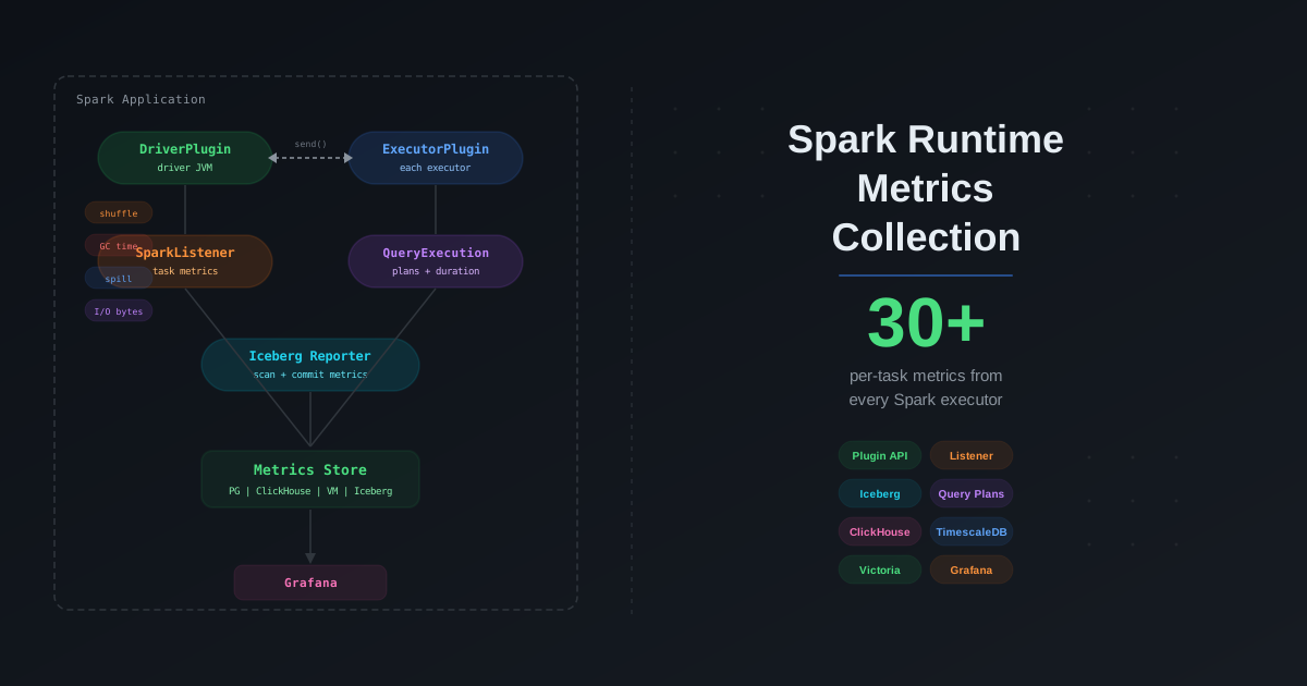
Apache Spark ships a powerful but underused plugin system — DriverPlugin, ExecutorPlugin, and SparkListener — that lets you tap into every metric the engine produces at runtime. Combined with Iceberg's MetricsReporter, you get a unified view of compute and storage performance for every query, every task, and every table scan. This post shows you how to build that pipeline from scratch, store the metrics at scale, and turn raw numbers into actionable performance insights.

You have a Spark job running on Iceberg tables. It works, but it is slow, expensive, or both. You have read a dozen blog posts about individual optimizations — broadcast joins, AQE, partition pruning, compaction — but you do not have a single place that tells you what to check, in what order, and what the correct configuration values are. Every tuning session turns into a scavenger hunt across documentation, Stack Overflow, and tribal knowledge.

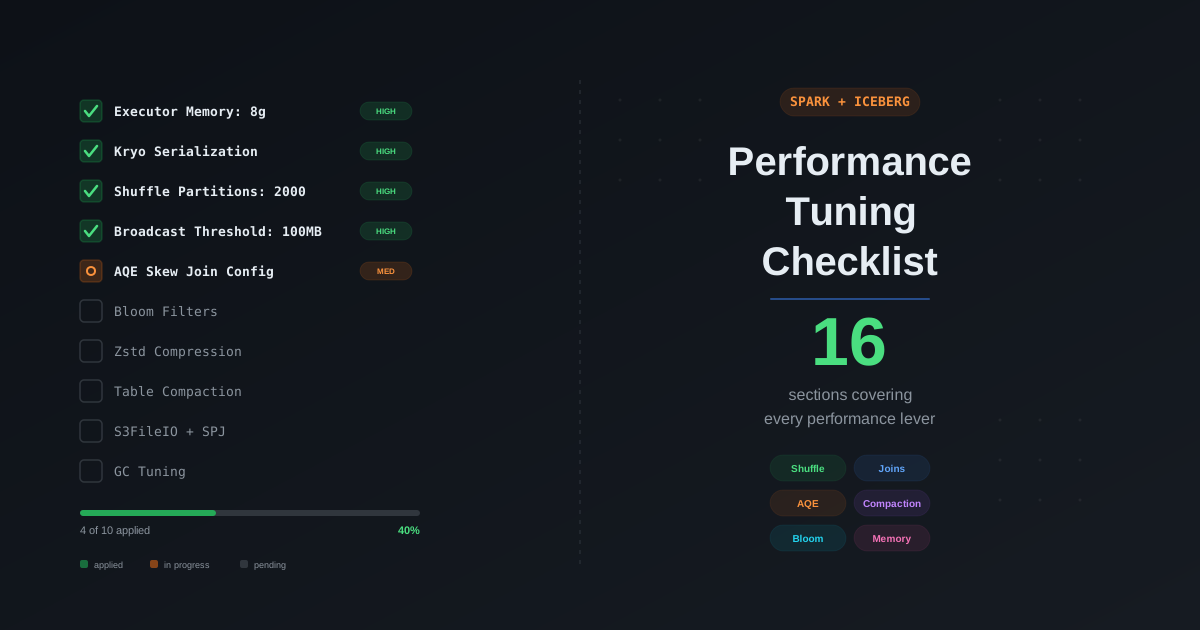
This post is the checklist you run through every time. We cover every performance lever in the Spark and Iceberg stack, organized from highest impact to lowest, with the exact configurations, recommended values, and links to our deep-dive posts for the full explanation. If you only have 30 minutes, work through the first five sections. If you have a day, work through all sixteen. Every item has been validated in production workloads on the Cazpian lakehouse platform.

Your Spark job runs for 45 minutes. You check the Spark UI and find that a single join stage consumed 38 of those minutes — shuffling 800 GB across the network because the optimizer picked SortMergeJoin for a query where one side was 40 MB after filtering. Nobody ran ANALYZE TABLE. No statistics existed. The optimizer had no idea the table was small enough to broadcast.

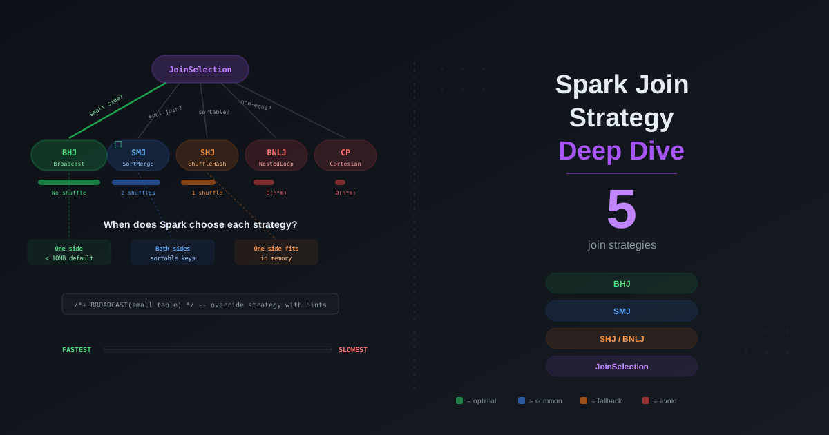
The join strategy is the single most impactful decision in a Spark SQL query plan. It determines whether your data shuffles across the network, whether it spills to disk, whether your driver runs out of memory, and whether your query finishes in seconds or hours. Spark offers five distinct join strategies, each with different performance characteristics, memory requirements, and failure modes. The optimizer picks one based on statistics, hints, configuration, and join type — and it often picks wrong when it lacks information.

This post covers every join strategy in Spark, how the JoinSelection decision tree works internally, how the Catalyst optimizer estimates sizes, how CBO reorders multi-table joins, every join hint and when to use it, how AQE converts strategies at runtime, the equi vs non-equi join problem, how to read physical plans, the most common anti-patterns, and a real-world decision framework you can use in production.

You have a 500 million row table in PostgreSQL. You write spark.read.jdbc(url, "orders", properties) and hit run. Thirty minutes later, the job is still running. One executor is at 100% CPU. The other 49 are idle. Your database server is pegged at a single core, streaming rows through a single JDBC connection while your 50-node Spark cluster sits there doing nothing.

This is the default behavior of Spark JDBC reads. No partitioning. No parallelism. One thread, one connection, one query: SELECT * FROM orders. Every row flows through a single pipe. It is the number one performance mistake data engineers make with Spark JDBC, and it is the default.

This post covers everything you need to know to fix it and to optimize every aspect of Spark JDBC reads and writes. We start with why the default is so slow, then go deep on parallel reads, all pushdown optimizations, fetchSize and batchSize tuning, database-specific configurations, write optimizations, advanced patterns, monitoring and debugging, anti-patterns, and a complete configuration reference.

Your 200-node cluster finished 199 of 200 tasks in 30 seconds. The last task has been running for 45 minutes. Every executor except one is idle, burning compute cost while it waits for a single partition containing 80% of the data to finish processing. The stage progress bar is stuck at 99.5%. Your Spark job that should take 2 minutes is taking an hour.

This is data skew -- the single most common and most destructive performance problem in distributed data processing. It turns a perfectly parallelized cluster into an expensive single-threaded computation. It wastes money, wastes time, and breaks SLAs. And it is entirely fixable once you know how to identify it and which optimization to apply.

This post goes deep on every dimension of data skew. We start with what it is and why it kills performance, show exactly how to identify it in the Spark UI, catalog every type of skew you will encounter, cover the AQE automatic optimizations that handle skew at runtime, walk through every manual fix with code examples, address Iceberg-specific skew problems, provide a complete configuration reference, and close with the anti-patterns that cause skew in the first place.

You are running the same 500 GB join three times in a single pipeline — once for a daily summary, once for a top-products report, once for customer segmentation. Each query reads from S3, shuffles terabytes across the network, builds hash maps, and aggregates from scratch. That is 1.5 TB of redundant I/O, three redundant shuffles, and three redundant sort-merge joins.

Spark caching eliminates this waste. You compute the expensive join once, store the result in executor memory, and every subsequent query reads from that in-memory copy instead of going back to object storage. The improvement is not incremental — it is typically 10-100x faster for repeated access patterns.

But caching does something else that is less obvious and equally powerful: it makes Spark's query optimizer smarter. When a table is cached, Spark knows its exact in-memory size. If that size falls below the broadcast join threshold, the optimizer automatically converts a Sort-Merge Join into a Broadcast Hash Join — eliminating the shuffle entirely, without you writing a single hint.

This post covers every dimension of Spark caching. We start with internals, walk through every storage level, show all the ways to cache, explain the columnar storage format that makes DataFrame caching special, dive into memory management, discuss how much data you should actually cache (spoiler: not terabytes), show you how to read the Spark UI Storage tab, and cover the pitfalls that catch production workloads.

Your 500-node Spark cluster is shuffling a 2 TB fact table across the network — serializing every row, hashing it, writing it to disk, sending it over the wire, and deserializing it on the other side — just to join it with a 50 MB dimension table. Every single query. Every single day.

The shuffle is the most expensive operation in distributed computing. It consumes network bandwidth, disk I/O, CPU cycles, and memory on every executor in the cluster. And for joins where one side is small, it is completely unnecessary.

Broadcast join eliminates the shuffle entirely. Instead of redistributing both tables across the cluster, Spark sends the small table to every executor, where it is stored as an in-memory hash map. Each executor then joins its local partitions of the large table against this hash map — no network shuffle, no disk spill, no cross-executor coordination. The result is typically a 5-20x speedup over Sort-Merge Join for eligible queries.

This post goes deep. We cover exactly what happens inside a broadcast join, all five ways to trigger one, how AQE converts joins at runtime, the real memory math that catches people off guard, when broadcast hurts instead of helps, and how to monitor and debug broadcast behavior in production.