18 posts tagged with "Cost & FinOps"

What lakehouse compute actually costs, and how to pay less for it.

View All Tags

We Moved Cazpian's Spark Pools to ARM — 2x Faster Under Load

· 12 min read

Cazpian Engineering
Platform Engineering Team

Cazpian Spark pools on Graviton ARM64: median job 5,109 ms vs 9,953 ms on x86 under 100-way concurrency

Conventional wisdom says migrating a data engine to ARM is a performance gamble you take for the discount. We ran the experiment on our own Spark compute pools, and the result inverted the premise: under 100-way concurrency, the ARM64 pool ran every job roughly twice as fast as its x86 twin — at about 20% lower infrastructure cost.

We are publishing the numbers, but also the part benchmark posts usually cut: our first measurement said ARM was 8.5x slower, and that number was wrong in a way that had nothing to do with ARM. If you are planning an ARM migration for your data platform, the detour is probably worth more to you than the table.

100 Concurrent Spark Jobs, 67 Seconds, One $2/Hour Pool

· 8 min read
Cazpian Engineering
Platform Engineering Team

100 concurrent Spark jobs, each scanning 200 MB, all finished in 67.5 seconds on one $2/hour pool

In The Small Job Tax we made an argument: most data platforms make you pay cluster-sized overhead for container-sized work, and your smallest jobs are quietly your most expensive per byte.

An argument is cheap. So we measured it.

One hundred Spark jobs, submitted concurrently, each one scanning ~200 MB of Iceberg data — 19 GiB of real columnar IO and 410 million rows in total — finished in 67.5 seconds, on one small compute pool that costs about $2 an hour. One hundred submitted, one hundred succeeded, zero failures.

Then we kept pushing: 200 jobs, 300, 400, 500. The pool never became the problem.

What a Terabyte Actually Costs: TPC-DS on Cazpian

· 15 min read
Cazpian Engineering
Platform Engineering Team

TPC-DS 1 TB on Cazpian

There is a long-standing assumption in data engineering: if you want fast SQL, you do not use Spark. Spark is for pipelines. For interactive analytics you bring in a dedicated query engine, run it alongside, and accept the cost of operating two systems over one set of tables.

We wanted to know how true that still is. So we ran the full TPC-DS benchmark — all 103 queries — against a terabyte of Apache Iceberg data on a four-worker Cazpian cluster, and published everything: every query time, the cost, the hardware utilisation, and the parts that are not yet good enough.

We Benchmarked Native Query Acceleration on Iceberg — Up to 4.14x, and the Version Number That Almost Fooled Us

· 14 min read
Cazpian Engineering
Platform Engineering Team

Native acceleration on Iceberg, measured

Every native execution engine for Spark arrives with the same headline: 2x, 3x, sometimes 5x faster. The benchmarks are usually real. What they rarely tell you is whether they describe your data, your table format, and your version matrix.

So we measured it ourselves. Cazpian Native Query Acceleration, against 200 million rows of Apache Iceberg data, on the Spark version we ship. We recorded wall-clock time, CPU seconds, peak memory, and — the part most benchmarks skip — whether the answers came back the same.

The result: 1.51x faster on 45% less CPU across a mixed suite, with every result identical to standard Spark. On decimal aggregation — the shape most finance and revenue reporting takes — 3.18x in the suite, and 4.14x when we later measured it end to end through the Iceberg catalog.

We also nearly published the exact opposite conclusion. Our first full round measured zero acceleration on Iceberg — not "a little", literally zero accelerated operators across five configurations. That result was real, reproducible, and completely misleading, and the reason it was wrong is worth more to you than the speedup number.

The Serverless Black Box: What You Lose on Databricks Serverless Compute

· 13 min read
Cazpian Engineering
Platform Engineering Team

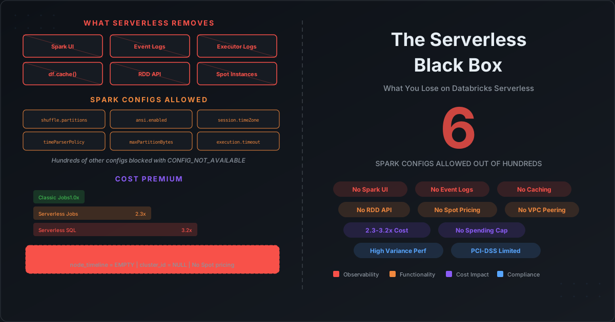
The Serverless Black Box: What You Lose on Databricks Serverless Compute

Databricks serverless compute promises a simple deal: stop managing clusters and just run your workloads. No instance selection. No autoscaling policies. No driver sizing. Just submit your query or job and let Databricks handle the rest.

The pitch is compelling. The reality is a black box that removes not just infrastructure management, but your ability to observe what is happening, tune how it runs, and control what it costs.

This is Part 3 of our Databricks observability series. In the previous post, we documented how system tables leave critical metrics gaps. Serverless makes those gaps dramatically worse — because on serverless, you lose even the tools that classic compute provides.

Databricks System Tables: The Observability Gap — What They Expose vs What You Actually Need for Cost Control

· 17 min read
Cazpian Engineering
Platform Engineering Team

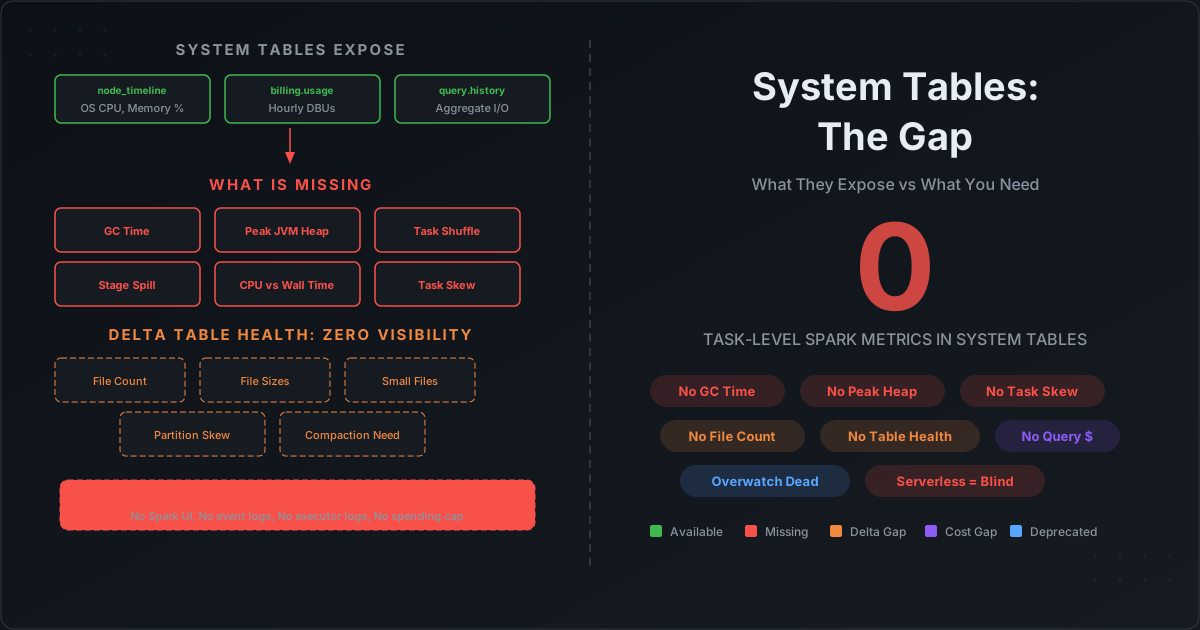
Databricks System Tables: The Observability Gap

Databricks system tables look comprehensive on paper. Sixteen tables across ten schemas. Billing, compute, jobs, queries, lineage, audit. When Databricks deprecated Overwatch and pointed everyone to system tables, the message was clear: this is the future of observability.

But if you have ever tried to answer these questions using only system tables, you already know the gap:

  • Why is my job's GC time at 15%? (System tables do not track GC time.)
  • Which stage is spilling to disk? (System tables do not track per-stage spill.)
  • Which executor is the memory bottleneck? (System tables do not track executor-level JVM metrics.)
  • How many files does my Delta table have? Is it healthy? (System tables do not track Delta table physical metrics.)
  • What did my serverless job's infrastructure look like? (System tables do not populate node_timeline for serverless.)

This post documents exactly what Databricks system tables contain — column by column — and exactly what is missing. Every claim is verifiable against Databricks' own documentation.

How to Profile Spark Jobs After Completion: The Complete Guide to Collecting Metrics on Databricks, EMR, and Dataproc

· 22 min read
Cazpian Engineering
Platform Engineering Team

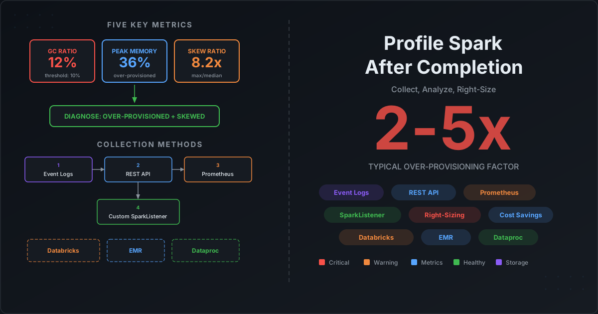
How to Profile Spark Jobs After Completion

Your Spark job finished. It ran for 2 hours. It used 50 executors. The bill arrived. Now what?

Most teams have no systematic way to answer the obvious follow-up questions: Was 50 executors the right number? Did we waste memory? Was there data skew? Should we use different instance types? They either overprovision "just in case" — burning 2-5x the needed budget — or reactively debug when jobs fail with OOM errors.

The root cause is not a lack of tooling. It is a data collection problem. Spark generates extraordinarily detailed metrics at every level — task, stage, executor, application — but those metrics vanish when the application terminates. If you did not capture them during or immediately after execution, they are gone.

This post solves that problem. We cover every method for collecting Spark profiling metrics, show exactly how to set them up on Databricks, EMR, and Dataproc, and then show you how to turn those metrics into right-sizing decisions with concrete formulas and thresholds.

Iceberg Scan and Commit Fine-Tuning: The Production Operations Guide for Spark

· 29 min read
Cazpian Engineering
Platform Engineering Team

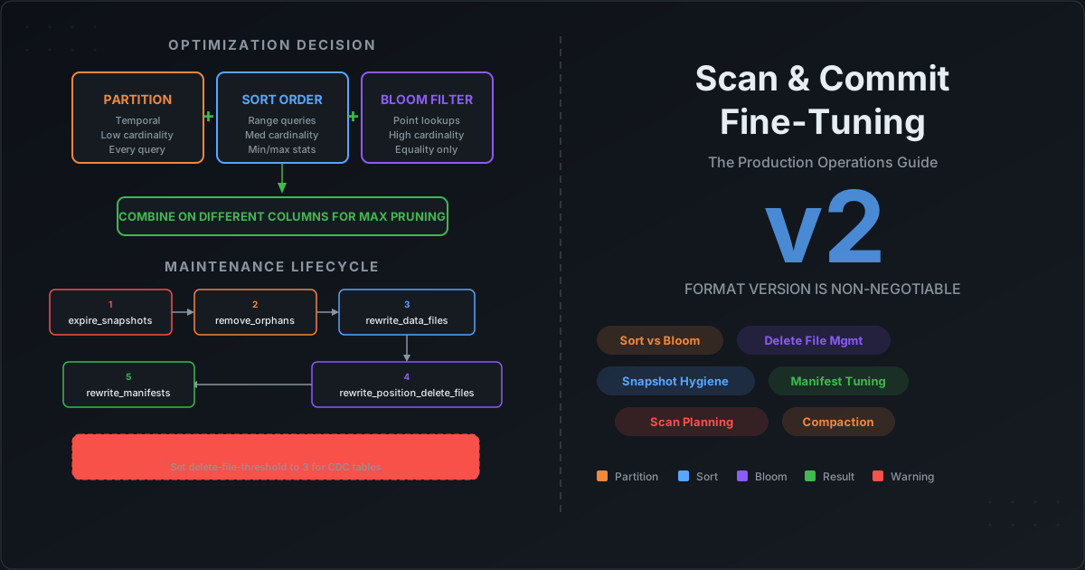
Iceberg Scan and Commit Fine-Tuning: The Production Operations Guide for Spark

You have set up your Iceberg tables. You picked a partition spec. You enabled bloom filters. Maybe you even ran compaction once. But the questions keep coming: Should I sort the table AND add bloom filters, or is one enough? My queries are still opening thousands of files — what is Spark actually doing during scan planning? I have 50,000 snapshots — is that a problem? I switched to format version 2 but my reads got slower — why? What happens if I never compact my delete files?

These are the questions that every data engineering team hits after the first month in production. The individual features are documented, but the interactions between them — and the operational decisions that determine whether your tables stay fast or silently degrade — are not written down anywhere.

This post is the production operations guide. We cover the decision framework for partition vs sort vs bloom filter, explain exactly what happens during scan planning so you know where compute is wasted, walk through every maintenance procedure with recommended thresholds, explain why format version 2 is non-negotiable and what delete file neglect costs you, and give you the complete maintenance lifecycle in the right execution order.

Iceberg Metrics Reporting: How to Monitor Scan and Commit Health with Spark

· 20 min read
Cazpian Engineering
Platform Engineering Team

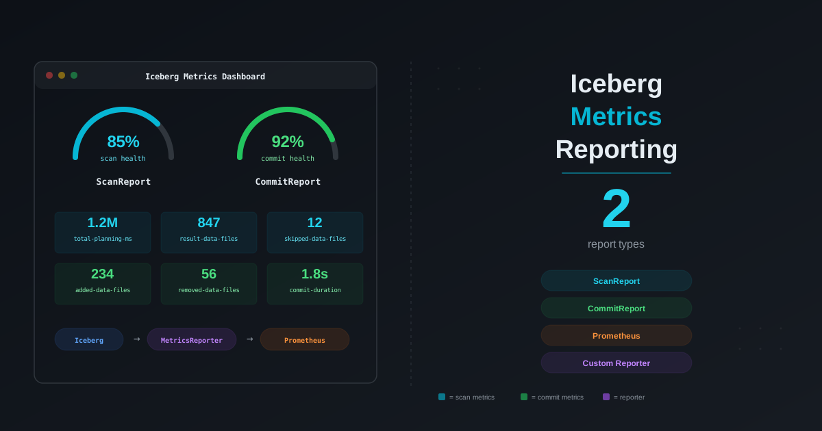
Iceberg Metrics Reporting: How to Monitor Scan and Commit Health with Spark

You designed the partitions correctly. You set up compaction. You even configured bloom filters. But your Iceberg tables are still slow — and you have no idea why. Is it the scan planning? Too many manifests? Delete files accumulating silently? Commit retries from writer contention? You cannot fix what you cannot see.

Apache Iceberg actually gives you everything you need to diagnose table health. The problem is that the metrics are scattered across six different layers — a Java API, virtual SQL tables, snapshot properties, file-level statistics, Puffin blobs, and engine-level instrumentation — and no one has assembled them into a single picture. This post does exactly that.

We will walk through every layer of Iceberg metrics, show you how to collect them, explain what each metric means for your read and write performance, and give you concrete thresholds and SQL queries that tell you when something is wrong and what to do about it.

Iceberg Bloom Filters with Spark: Configuration, Validation, and Performance Guide

· 21 min read
Cazpian Engineering
Platform Engineering Team

Iceberg Bloom Filters with Spark: Configuration, Validation, and Performance Guide

When you query an Iceberg table with WHERE user_id = 'abc-123', Spark reads every Parquet file that could contain that value. It first checks partition pruning — does this file belong to the right partition? Then it checks column statistics — does the min/max range for user_id in this file include 'abc-123'? But for high-cardinality columns like UUIDs, user IDs, session IDs, or trace IDs, min/max statistics are nearly useless. The min might be 'aaa...' and the max might be 'zzz...', so every file passes the min/max check even though only one file actually contains the value.

This is where bloom filters come in. A bloom filter is a compact probabilistic data structure embedded in each Parquet file that can definitively say "this value is NOT in this file" — allowing Spark to skip the file entirely. For point lookups on high-cardinality columns, bloom filters can reduce I/O by 80-90%.

This post covers everything you need to know: how bloom filters work internally, when to use them, how to configure them on Iceberg tables, how to validate they are present in your Parquet files, and what false positives mean for your data correctness.

Storage Partitioned Joins in Apache Iceberg with Spark

· 13 min read
Cazpian Engineering
Platform Engineering Team

Storage Partitioned Joins in Apache Iceberg with Spark

Every Spark join starts the same way: read both sides, shuffle the data across the network so matching keys end up on the same executor, then join. That shuffle is the single most expensive operation in most Spark jobs — it moves data across the network, writes temporary files to disk, and consumes memory on every executor in the cluster.

But what if both tables are already organized by the join key on disk? If the left table's customer_id=42 rows are in bucket 42 and the right table's customer_id=42 rows are also in bucket 42, there is nothing to shuffle. Each executor can join its local partitions independently.

That is exactly what Storage Partitioned Join (SPJ) does. Introduced in Spark 3.3 and matured in Spark 3.4+, SPJ is the most impactful — and least understood — optimization available for Iceberg+Spark workloads. This post shows you how it works, how to set it up, how to verify it, and where it breaks.

Iceberg on AWS: S3FileIO, Glue Catalog, and Performance Optimization Guide

· 20 min read
Cazpian Engineering
Platform Engineering Team

Iceberg on AWS: S3FileIO, Glue Catalog, and Performance Optimization Guide

If you are running Apache Iceberg on AWS, the single most impactful configuration decision you will make is your choice of FileIO implementation. Most teams start with HadoopFileIO and s3a:// paths because that is what their existing Hadoop-based stack already uses. It works, but it leaves significant performance on the table.

Iceberg's native S3FileIO was built from the ground up for object storage. It uses the AWS SDK v2 directly, skips the Hadoop filesystem abstraction entirely, and implements optimizations that s3a cannot — progressive multipart uploads, native bulk deletes, and zero serialization overhead. Teams that switch typically see faster writes, faster commits, and lower memory usage across the board.

This post covers everything you need to run Iceberg on AWS efficiently: why S3FileIO outperforms s3a, how to configure every critical property, how to avoid S3 throttling, how to set up Glue catalog correctly, and how to secure your tables with encryption and credential vending.